What is Dollar-Cost Average?
Investors sometimes like to use the Dollar-Cost Average (or Dollar-Cost Averaging, DCA) buying strategy when purchasing stock. DCA is just a fancy way to say that instead of buying a security all at once, you want to split up your purchases into multiple buys at different times, typically with the hope that you will ultimately have a lower average cost than if you had otherwise just purchase all the shares you desired up front. The question is, how do you calculate what your average cost per share is?
File companion:
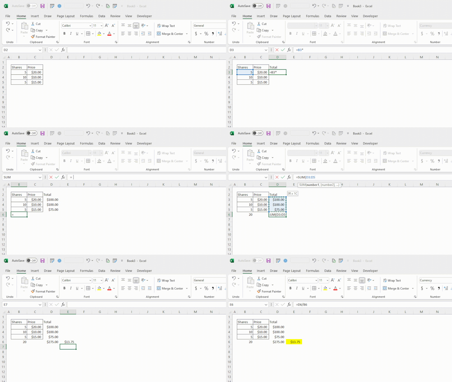
To determine your dollar cost average, you need to determine the weighted averaged cost of the shares you purchased. This means that you take into consideration the number of shares purchased, rather than just the price of each individual buy. Something like this:
DCA = (total cost of shares) / (total shares purchased)
Take for example you're buying shares of XYZ. Here are your purchases:
5 shares @ $20 each
10 shares @ $10 each
5 shares @ $15 each
While your purchase price was an average of $15 (20 + 10 + 15) / (3 total buys), this is in fact not the DCA. The weighted average price or the DCA needs to factor in the number of shares bought at each price, so in this case would be as follows:
(5 * $20 + 10 * $10 + 5 * $15) / 20 shares = $13.75

Now let's look at a couple options of how to do this a little faster with less intermediate steps.
Option 1: Weighted Average Excel Formula
Bad news: Unfortunately, Excel does not have a built in weighted average function.
Good news: That doesn't mean we can't build one ourselves!
To build a weighted average or DCA formula, we'll really only need two functions: We'll use SUMPRODUCT to calculate the total investment, and SUM to just get the total shares purchased. Consider you have data like this:
| A | B | C |
1 | Date | Shares | Price |
2 | 6/8/2021 | 33 | $11.40 |
3 | 6/9/2021 | 64 | $13.83 |
4 | 6/10/2021 | 70 | $12.30 |
5 | 6/11/2021 | 63 | $10.96 |
We can use the SUMRPODUCT function here to skip the step of calculating each day's total. All we need to enter in this case is:
=SUMPRODUCT(B2:B5,C2:C5)
SUMRPODUCT works by taking two ranges, multiplying each line together, and adding up the results, exactly the same as the previous example, with less steps! Now that we got the total investment down, we just have to divide by the total shares, like this:
=SUMPRODUCT(B2:B5,C2:C5)/SUM(B2:B5)And viola! there's your DCA in Excel.
Option 2: Creating a Custom DCA Function with LAMBDA
If you find that you have a worksheet where you are setting this up often, it might be worth adding a custom LAMBDA function to your file. LAMBDA allows you to take a formula like the one that we just set up, name it, and use it wherever you want in your workbook. Note that this portion requires Excel 365.
When you're looking to convert a formula to a named function with LAMBDA, you need to think about what your inputs and output will be. In this case, we have the range of prices and range of quantities, and we want our function to return simply the DCA of these values. We start by wrapping our current formula in a LAMBDA function and then replace each reference with input at the beginning of the function:
=LAMBDA(SUMPRODUCT(B2:B5,C2:C5)/SUM(B2:B5))
=LAMBDA(pricesRange,SUMPRODUCT(B2:B5,pricesRange)/SUM(B2:B5))(C2:C5)
=LAMBDA(pricesRange,quantitiesRange,SUMPRODUCT(quantitiesRange,pricesRange)/SUM(quantitiesRange))(C2:C5,B2:B5)
When creating and running an un-named LAMBDA like what we just created, the trick is to throw the inputs to the LAMBDA at the end of the formula, wrapped in parentheses. Now that we've made the LAMBDA, we can name it in the name manager in the following steps:
Copy the entire LAMBDA formula without the input at the end: =LAMBDA(pricesRange,quantitiesRange,SUMPRODUCT(quantitiesRange,pricesRange)/SUM(quantitiesRange))
In the Formulas Tab, open the Name Manager. Alternatively, press Ctrl + F3. Click New...
Type DCA in the "Name" section. Paste the formula in the "Refers to" box. You can also give the formula a description that will appear when someone is writing the formula in a cell.
Hit ok and go test your new custom function!

I hope you found this helpful and learned something new! Please feel free to leave questions in the comments below, and be sure to subscribe to be notified of future posts!
